Using Pandoc and knitR with Sphinx
This is a short example illustrating how to use knitr with pandoc to write a single document in markdown and have it rendered in multiple formats, especially pdf and html. For the purposes of illustration, I have chosen two code chunks, one generating a plot and the other generating a table to illustrate the power of pandoc + knitr.
We first need to tell knitr to render the output of code chunks in the gfm format, which pandoc will understand.
The chunk below is a plot chunk. You need to have the package ggplot2 installed for it to work.
library(ggplot2)
qplot(wt, mpg, data = mtcars)
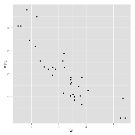
plot of chunk plot-chunk
The second chunk produces a table. You need to have the package ascii installed for this to work.
library(ascii)
x <- head(mtcars[, 1:5])
options(asciiType = "pandoc")
ascii(x)
| mpg | cyl | disp | hp | drat | |
|---|---|---|---|---|---|
| Mazda RX4 | 21.00 | 6.00 | 160.00 | 110.00 | 3.90 |
| Mazda RX4 Wag | 21.00 | 6.00 | 160.00 | 110.00 | 3.90 |
| Datsun 710 | 22.80 | 4.00 | 108.00 | 93.00 | 3.85 |
| Hornet 4 Drive | 21.40 | 6.00 | 258.00 | 110.00 | 3.08 |
| Hornet Sportabout | 18.70 | 8.00 | 360.00 | 175.00 | 3.15 |
| Valiant | 18.10 | 6.00 | 225.00 | 105.00 | 2.76 |